How to Experiment Rapidly Without Losing Rigour

Posted by Harry Salmon & Mahana Mansfield on Monday, October 22, 2018

As data scientists at Deliveroo we evaluate our work via robust experimentation, and we take a frequentist hypothesis testing approach. The standard method places a lot of importance on deciding upfront how large an impact we believe any experiment might have. If the estimated impact is very different to the actual impact, we might waste a lot of time running an experiment where we could have obtained a result sooner. This means that we can’t iterate and innovate as quickly as we would like. Our preferred solution to this problem is sequential experiment designs.

Frequentist hypothesis testing: standard method

We have two populations \(A\) and \(B\), and the null hypothesis \(H_0\) is that the population means \(\mu_A\) and \(\mu_B\) are the same. The alternative hypothesis \(H_1\) is that these population means are different.

We run our experiment to try to find evidence that the null hypothesis is false. To do this we collect two sets sampling our populations \(X_A \subset A\), \(X_B \subset B\), and calculate the difference between the sample means \(\overline{X_A}\) and \(\overline{X_B}\). We then calculate the probability of observing a difference between sample means of the observed size or greater, in the case where the null hypothesis is true.

For any given experiment (or indeed for all our experiments as a whole) we decide on a maximum proportion of false positives (type I errors) that we will accept \(\alpha\) (often 0.05), and a maximum rate of false negatives (type II errors) that we will accept \(\beta\) (often 0.2). Our experimental power is defined as \(1 - \beta\) (and is therefore often 0.8). From these we are able to design a fixed sample size experiment capable of detecting a minimum difference between the population means of \(\delta_{detectable}\), with \(N_{Fixed}\) samples in each group.

This fixed sample size is inversely proportional to the square of the size of the effect we are trying to detect (assuming we keep \(\beta\) constant):

\(N_{Fixed} \propto \delta_{detectable}^{-2}\),¹

therefore as we aim to have more sensitive tests (i.e. we can detect smaller values of \(\delta\)), the sample size needed for experiments grows quickly.

A consequence of this is that, if we were to set a test running with an experiment design that is capable of detecting a very small \(\delta_{detectable}\), and in fact \(\delta\) is much larger, we will end up running the test for much longer than would be necessary.

This will either:

slow the process of finding a positive result, resulting in showing the old, inferior version to the control group for longer
or worsen the experience for users in the treatment group for an unnecessarily long time in order to gain confidence that the new experience is in fact worse.

In either case, we are slowing the pace of innovation.

We would ideally be able to check our experiment results while the experiment is still running to see if there is a very large result in either direction, but doing this without further work loses statistical rigour as we would be checking the results many times: this is the multiple comparisons problem.

These factors put a lot of pressure on what we decide up front as the difference between the two groups we want to be able to detect. It is a difficult quantity to come to a decision on, ideally the test would be as sensitive as possible to detect the actual difference and no more.

We want to run the same tests more rapidly, with fewer users, and be confident we’re not having a negative effect or that we are having a positive effect as early as possible.

Sequential testing

The sequential testing procedure takes the concept of a family-wise error rate² and applies it to multiple hypothesis tests across the duration of the experiment. By adjusting the threshold value \(\alpha\) at which we will reject the null hypothesis at each of the test’s checkpoints, we can maintain the total (i.e. family-wise) probability of making one or more type I errors at a desired level, \(\alpha_{T}\).

The trade-off is that, by spreading the errors across multiple checkpoints, we need to increase the maximum sample size for the sequential test to \(N_{Sequential} > N_{Fixed}\) in order to maintain \(\beta\).

In the case that our \(\delta_{detectable}\) estimate is very close to the true value of \(\delta\), the sequential design would increase the sample size required for our tests from \(N_{Fixed}\) to \(N_{Sequential}\). In many cases though we don’t have a good a priori estimate of the value of \(\delta\), so to make running the test worthwhile we often err on the side of being able to detect a slightly smaller effect than it may actually have, and thus running the test a bit longer. By introducing checkpoints we are able to set \(\delta_{detectable}\) to be quite small, but if the true value of \(\delta\) is larger we are likely to be able to stop running our test early, i.e. with a sample size less than \(N_{Sequential}\) (and likely less than \(N_{fixed}\)).

In designing a sequential experiment we need to additionally decide the following:

How often we want conduct hypothesis tests, i.e. select “checkpoints” \(N_{1}^{Sequential},N_2^{Sequential},...,N_k^{Sequential}\) with \(\sum_{i=1}^k N_i^{Sequential}=N_{Sequential}\)
How we want to distribute (also called “spend” or “split”) the type I and type II errors throughout the experiment, i.e. select \(\alpha_1,\alpha_2,\dots,\alpha_k\) and \(\beta_1,\beta_2,\ldots,\beta_k\) corresponding to the above checkpoints.

From these \(\alpha_i\) and \(\beta_i\) it is possible to create boundary values for the test statistic \(S_k\) at each checkpoint such that if it falls outside of a certain value, we can stop the test and declare a winner.

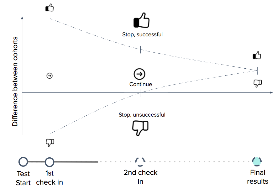
This image (generated using gsDesign) shows a two sided sequential test design where we have found upper \(u_k\) and lower \(l_k\) boundaries for the \(Z\) test statistic \(Z_k\) at each checkpoint from a set of \(\alpha_k\), \(\beta_k\). If the test statistic falls outside of these boundaries at any checkpoint then we can stop the test early. Derivation of these boundaries is covered below.

In theory we could decide on our checkpoints and how to distribute our errors after the beginning of our experiment, but in doing so we must be careful to not look at any data already gathered, so it is good practice to do this before the experiment starts.

The decision of how we want to distribute our type I and type II errors throughout the experiment is up to us, contingent on not increasing their totals. However, it makes some intuitive sense to have the greatest chance of detecting the effect at the point at which we have the most information from which to make this decision. As a result this will help keep \(N_{Sequential}\), \(N_{Fixed}\) similar, and avoid a large increase in the maximum sample size required for the experiment. With this in mind, a number of ways to determine suitable values of \(\alpha_i\) and \(\beta_i\) have been proposed ³. Many rely on fixed spacing of analysis (i.e. \(N_i^{Sequential} - N_{i-1}^{Sequential}\) is the same for all \(i\)), however, by using “error spending functions” we can generalise to any position of the checkpoints, and still maintain the desired properties of the test⁴⁵.

One method is to distribute the \(\alpha\) according to the fraction of information gathered at the point of that analysis⁴. This fraction of total statistical information gathered is referred to in the literature as the information fraction, and for normally distributed data this information fraction is equal to the proportion of data gathered, \(\frac{N_i}{N_{Sequential}}\)⁴. Following this, we can choose values of \(\alpha\) according to:

\[\alpha_i=\alpha_T\frac{N_i}{N_{Sequential}}^p\]

where the increment \(\alpha_i - \alpha_{i-1}\) represents the additional amount of alpha or type I error probability that can be used at the kth analysis³.

The value of \(p\) controls how conservative the boundaries should be at the early versus late analyses⁵, with higher values of \(p\) being more conservative early in the test.

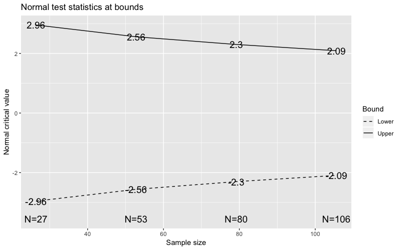
In keeping with the recommendation in “Efficient A/B Testing in Conversion Rate Optimization”⁶, an upper boundary spending function as above with \(p=2\) achieves the compromise that if we see a very large improvement early we can roll out the change immediately, but without a large increase in \(N\) compared to the non sequential design.

Stopping early if success is unlikely

We can take the same approach to try to stop the test early if the value of the test statistic indicates that it is unlikely that we will find a winner (i.e. a significant difference between the groups) by the end of the test. This will allow us to stop unpromising tests earlier.

From the same approach as above we can calculate a set of values for \(\beta\):

\[\beta_i=\beta_T\frac{N_i}{N_{Sequential}}^p\]

This allows us to calculate an additional boundary also enabling early stopping of the experiment in the detrimental case, while still maintaining the same total type II error rate.

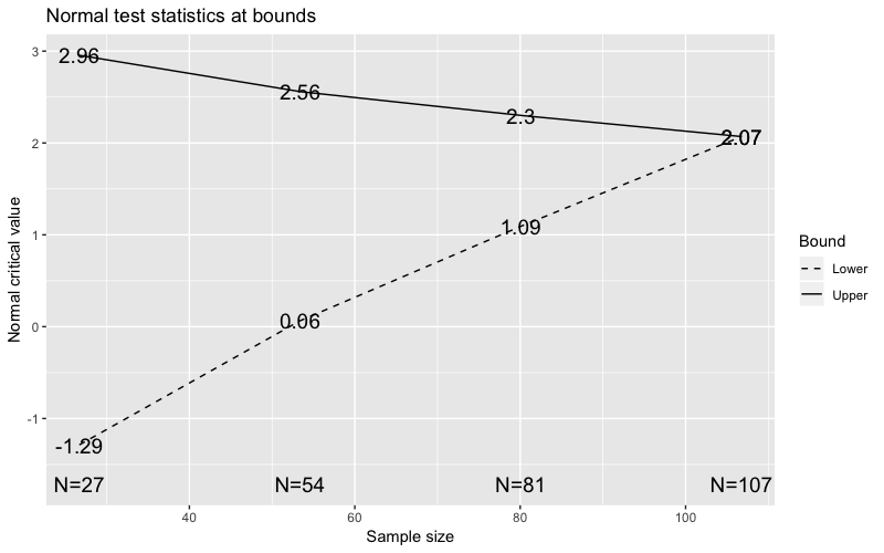
Again in line with the recommendations in “Efficient A/B Testing in Conversion Rate Optimization”⁶ we have chosen a value of \(p = 3\) for the lower boundary: it makes sense to be more conservative earlier on with the stopping criteria of the lower boundary for unsuccessful tests. As effort has been made in implementing the variant, if it is not having a significantly negative effect it is worth continuing the test for longer and not stopping very early on.

The following image shows a sequential design with an early stopping boundary and the same other design parameters as above. So as before if our test statistic \(S_k\) falls outside of the bounds at any of the checkpoints we can stop the test, either declare a winner or no winner, and reduce the total sample size needed.

Determining the boundaries

For a given test statistic \(S\) (for example the \(Z\) statistic used above), the upper and lower boundaries must fit the following constraints⁴:

Under the null hypothesis the probability of the test statistic \(S_1\) being greater than or equal to the value of the upper boundary at the first checkpoint must be equal to the alpha spending function at the first checkpoint: \(P_{H_0}(S_1 \geq u_1) = \alpha_T\frac{N_1}{N_{Sequential}}^p\).
Under the alternative hypothesis in the case where the true difference between groups is exactly the minimum detectable difference, the probability of the test statistic being less than the lower boundary at the first checkpoint must equal the beta spending function at the first checkpoint: \(P_{H_1}(S_1 \leq l_1) = \beta_T\frac{N_1}{N_{Sequential}}^p\).
Under the null hypothesis the probability that the test statistic falls between the two boundaries \(l_1 \leq S_1 \leq u_1\) at all previous boundaries and then falls above the upper boundary \(u_k\) at the \(k\)-th analysis must be equal to the difference between the alpha spending function at the \(k\)-th boundary and the spending function at the previous checkpoint: \(P_{H_0}(l_1 \leq S_1 \leq u_1, \ldots , l_{k-1} \leq S_{k-1} \leq u_{k-1},S_k\geq u_k) = \alpha_T\frac{N_k}{N_{Sequential}}^p - \alpha_T\frac{N_{k-1}}{N_{Sequential}}^p\).
Under the alternative hypothesis as before, the probability that the test statistic \(S_1\) falls between the two boundaries \(l_1 \leq S_1 \leq u_1\) at all previous boundaries and then falls below the lower boundary at the \(k\)-th analysis must be equal to the spending function at the \(k\)-th boundary: \(P_{H_1}(l_1 \leq S_1 \leq u_1, \ldots , l_{k-1} \leq S_{k-1} \leq u_{k-1},S_k\leq l_k) = \beta_T\frac{N_k}{N_{Sequential}}^p - \beta_T\frac{N_{k-1}}{N_{Sequential}}^p\).

By satisfying these constraints we can find the amount by which we must increase the sample size of the experiment \(N_{Sequential}\) in order to maintain \(\alpha_T\) and \(\beta_T\). We are also then able to reposition the checkpoints \(N\) and find the appropriate upper and lower boundary values for these checkpoints. These equations must be solved numerically⁵⁴.

Our current sequential design

Using the \(Z\) test statistic we have taken the above spending function with \(p=2\) for the upper boundary and \(p=3\) for the lower (futility) boundary as mentioned earlier. We have decided to check the test at 10% of the samples, 50% and 100%. For a two tailed test with \(\alpha_T= 0.05\) and \(\beta_T=0.2\) this gives the design shown below. We need to consider the below image also mirrored around zero for the negative case.

Here is a worked R code example:

# delta := how small is the difference we are trying to detect

install.packages('gsDesign'); require(gsDesign)
# past data on the variable of interest, from which to estimate the
# mean and standard deviation of the experimental data we will collect
data = rnorm(777, mean = 5, sd = 1)

s = sd(data)
delta = 0.1

# calculate the sample size which would be required for the
# standard design
n_fixed = power.t.test(n = NULL, delta, s,
                       sig.level = 0.05,
                       power = 0.8,
                       alternative = "two.sided")$n

# initital gsDesign object with evenly spaced checkpoints,
# used to calculate the maximum samples we would require
design = gsDesign(k=3, test.type = 4, alpha = 0.025, 
         sfu=sfPower, sfupar = 2, sfl=sfPower, 
         sflpar=3, n.fix = n_fixed,   beta = 0.2)

# the maximum number of samples which would be required for the
# sequential design
n_sequential = tail(design$n.I, 1)

# checkpoints at which we wish to check the experiment. E.g. at 10%
# 50%, and 100% of the maximum samples
checkpoints = c(
  ceiling(n_sequential / 10),
  ceiling(n_sequential / 2),
  ceiling(n_sequential)
)

# another gsDesign object which has our chosen checkpoints
gsDesign(k=3, test.type = 4, alpha = 0.025, sfu=sfPower, 
         sfupar = 2, sfl=sfPower, sflpar=3, n.fix = n_fixed,  
         n.I = checkpoints, beta = 0.2)

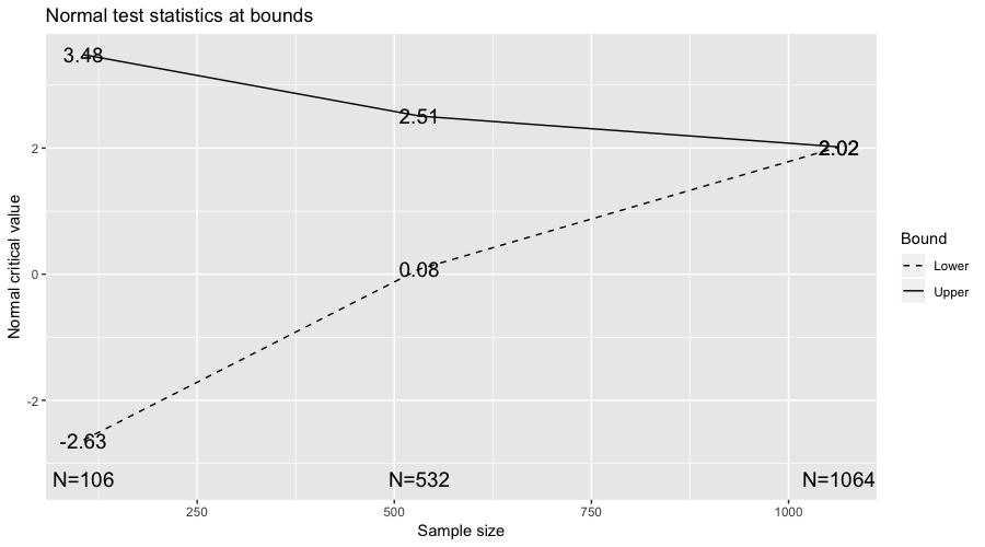
For a given sequential design the sample size required at the final checkpoint is a multiple of the fixed sample size design. The increase in the maximum sample size needed for this sequential design compared to the fixed design in this case is

\(N_{Sequential}=1.064 \cdot N_{Fixed}\).

We can see that the critical value of \(Z\) at the first upper boundary is 3.48 corresponding to a critical value of \(\alpha\) of 0.00025. For the two tailed test consider \(\alpha_T= 0.025\) for the upper boundary, from

\[\alpha_1=0.025 \cdot \frac{106}{1064}^2= 0.00025\]

we can see this satisfies our first constraint. The R package gsDesign⁷ was used to generate these sequential designs.

Summary

Sequential designs allow us to run flexible experiments, where the importance of estimating an accurate effect size upfront is reduced. They allow us to stop an experiment early if the true effect is larger than the estimated effect, which reduces wasted time and allows us to iterate and innovate quickly.

If you’re fascinated by sequential designs, come join our data science team!

Footnotes

HyLown Consulting LLC, G. (2018). Compare 2 Means 2-Sample, 2-Sided Equality | Power and Sample Size Calculators | HyLown. Retrieved from http://powerandsamplesize.com/Calculators/Compare-2-Means/2-Sample-Equality ↩
Wikipedia contributors. (2018, August 22). Family-wise error rate. In Wikipedia, The Free Encyclopedia. Retrieved 15:43, September 25, 2018, from https://en.wikipedia.org/w/index.php?title=Family-wise_error_rate&oldid=856111993 ↩
Demets, D., & Lan, K. (1994). Interim analysis: The alpha spending function approach. Statistics In Medicine, 13(13-14), 1341-1352. Retrieved from https://eclass.uoa.gr/modules/document/file.php/MATH301/PracticalSession3/LanDeMets.pdf ↩ ↩²
Sandro Pampallona, Anastasios A. Tsiatis, KyungMann Kim, 2001. (2018). Interim Monitoring of Group Sequential Trials Using Spending Functions for the Type I and Type II Error Probabilities. Retrieved from http://journals.sagepub.com/doi/abs/10.1177/009286150103500408 ↩ ↩² ↩³ ↩⁴ ↩⁵
Mark A. Weaver (2009). An Interim Analysis Example. Retrieved from http://www.icssc.org/Documents/AdvBiosGoa/Tab%2025.00_InterimAnalysis.pdf ↩ ↩² ↩³
Georgiev, G. (2018). Efficient A/B Testing in Conversion Rate Optimization: The AGILE Statistical Method. Retrieved from [https://www.analytics-toolkit.com/pdf/Efficient_AB_Testing_in_Conversion_Rate_Optimization_-The_AGILE_Statistical_Method_2017.pdf](https://www.analytics-toolkit.com/pdf/Efficient_AB_Testing_in_Conversion_Rate_Optimization-_The_AGILE_Statistical_Method_2017.pdf) ↩ ↩²
Anderson, K. (2016). Package ‘gsDesign’. Retrieved from https://cran.r-project.org/web/packages/gsDesign/gsDesign.pdf ↩

About Harry Salmon

Harry is a data scientist at Deliveroo. When not science-ing data he can usually be found climbing rocks.

About Mahana Mansfield

I always thought I’d be a mathematician, but turned to data science in 2011 shortly after finishing my PhD in algebraic topology. Since then I’ve had great fun doing data science and latterly leading data science teams. When I’m not doing data science, you can probably find me on the judo mat, in the gym trying to improve my Olympic lifting, or reading a never ending stream of health and exercise blogs/papers/books.