Monte Carlo Power Analysis
Take advantage of computing power and empirical data to use Monte Carlo simulation to perform experiment power analysis.
Experimentation is a key part of shipping new features here at Deliveroo. Each of our product teams has an embedded data scientist to help design the experiments and analyse the results. When we have a new feature to ship, we will design an experiment to test if it improves a small number of pertinent metrics. We will need to decide what metrics we will be tracking and how we define success of an experiment.
Prior to starting an experiment, the data scientist will have to ask a number of questions:
- What is the minimum effect size (change in our metric) that we want to be able to detect?
- What sample size do we need in order to have a good chance of detecting this minimum effect size?
Obtaining an answer to the second question is called Power Analysis. Deciding the minimum effect size is often a business judgement and is an input into Power Analysis. Usually we only have to answer one of these questions: we choose the minimum effect size and need to calculate the sample size (duration of the experiment) or we have a fixed sample size and observe the minimum effect size that we expect would give us a significant result. While there are a number of online calculators and analytical methods (closed-form) to help us do this, we find using Monte Carlo simulation is far more flexible when running experiments with different designs and potentially multiple metrics. In this blog post we will talk through how and why to use Monte Carlo simulation for power analysis and briefly introduce our internal experimentation framework Echidna.
What is statistical power?
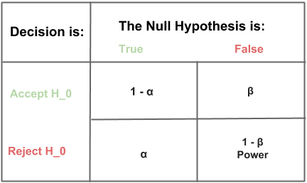
When measuring the impact of an experiment we are deciding if the average outcome in the variant is significantly different from the average outcome in the control, and we use frequentist hypothesis testing approaches to determine that. The statistical power of an experiment for a given alternative hypothesis is the probability we will get a statistically significant result (reject the null hypothesis) when the alternative is true:
\[power = 1 - \beta = P(\textrm{Reject }H_0|H_1\textrm{ is true})\]A result is determined to be statistically significant if the observed effect was unlikely to have been seen by random chance. How unlikely is determined by the significance level, \(\alpha\), that is the likelihood of rejecting the null hypothesis given it is true:
\[\alpha = P(\textrm{Reject }H_0|H_0\textrm{ is true})\]We will set \(\alpha\) and \(power\) before we begin our power analysis. Common settings for \(\alpha\) and \(power\) are 5% and 80% respectively. We are free to set \(\alpha\) and \(power\) depending on the level of confidence we would prefer in our business context. The table below shows the relationship between \(\alpha\) and \(power\), sometimes called a Truth Table.
Once we decide on our experimental design, pertinent metric(s), andpower, we will need to decide a minimum effect size then use power analysis to determine our required sample size. We may additionally use sequential experiment design, but we always require an initial fixed sample size to determine our sequential checkpoints.
Why not use analytical power analysis?
Analytical functions for performing power analysis for most common statistical tests are available in R and Python. We have found three limitations in using these libraries:
-
For experiments with multiple comparisons, it may not be possible to use analytical methods. In a simple case of multiple variants with the same sample size per variant, we can use a Bonferroni correction and plug the adjusted alpha into an analytical method. In anything more complicated (unequal sample sizes per variant, multiple metrics where we care about the probability that one metric is significant, etc.) Monte Carlo simulation is likely our only choice.
-
Our data is often distributed in non-standard ways (non-Normal, non-Bernoulli, etc.) and contains outliers. This will almost certainly violate some of the assumptions of the statistical test, particularly when we are aggregating our experimental units and consequently dealing with relatively small sample sizes. Violating these assumptions doesn’t mean we cannot use the statistical test but it will reduce our power. Using Monte Carlo simulation we can generate samples from the empirical distribution of our previous data and understand the sample size required to reach power given the distribution of our actual data.
-
Monte Carlo simulation allows us to have a standard way of performing power analysis regardless of the experiment design used. Prior to launching an experiment, we may want to quickly iterate our experiment design, for example compare the sample size needed for a randomised block design versus a randomised block design where we control for day of week and geographic effects. It may be possible to use analytical power analysis methods for both, but often this will require research and checking of assumptions to find the right analytical methods. With Monte Carlo simulation we can iterate much faster.
Using Monte Carlo simulation for Power Analysis
Now that have an understanding of why we want to use Monte Carlo simulation for power analysis let’s look at an example of how we would do it. The initial steps are:
- Collect sample data of the metric(s) we are influencing in the experiment over a fixed period of time.
- Inspect the sample data and decide on the statistical test that is appropriate for this data (t-test, Chi-Squared, etc.).
Once we have our data, we have provided an example below in Python of how to run the Monte Carlo simulation:
import numpy as np

from scipy.stats import norm, binom
from statsmodels.stats.weightstats import ttest_ind

# Sample data would be actual data measured over a fixed period of time prior to our
# experiment. For illustration purposes here we have generated data from a normal
# distribution.
sample_mean = 21.50
sample_sd = 12.91
sample_data = norm.rvs(loc=sample_mean, scale=sample_sd, size=20000)

sample_sizes = range(250, 20000 + 1, 250) # Sample sizes we will test over
alpha = 0.05 # Our fixed alpha
sims = 2000 # The number of simulations we will run per sample size
# The minimum relative effect we will test for (3%). We could try multiple relative
# effect is we are not sure what our minimum relative effect should be
relative_effect = 1.03
alternative = "two-sided" # Is the alternative one-sided or two-sided

power_dist = np.empty((len(sample_sizes), 2))
for i in range(0, len(sample_sizes)):
    N = sample_sizes[i]

    control_data = sample_data[0:N]
    # Multiply the control data by the relative effect, this will shift the distribution
    # of the variant left or right depending on the direction of the relative effect
    variant_data = control_data * relative_effect

    significance_results = []
    for j in range(0, sims):
        # Randomly allocate the sample data to the control and variant
        rv = binom.rvs(1, 0.5, size=N)
        control_sample = control_data[rv == True]
        variant_sample = variant_data[rv == False]

        # Use Welch's t-test, make no assumptions on tests for equal variances
        test_result = ttest_ind(control_sample, variant_sample,
                                alternative=alternative, usevar='unequal')
        # Test for significance
        significance_results.append(test_result[1] <= alpha)
    # The power is the number of times we have a significant result
    # as we are assuming the alternative hypothesis is true
    power_dist[i,] = [N, np.mean(significance_results)]
The Monte Carlo power analysis is shown visually below. Each data point represents a sample size tried, to generate each datapoint we have run 2000 simulations. The relative effect size has been set to 3%.
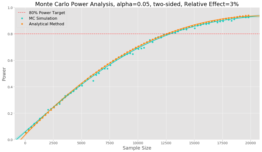
We would call this our power curve. To make it easier to see where we reach our power target we fit a polynomial regression to the data points. In this example we see our simulation gives the same sample sizes as the analytical method.
The power curve shows us that, based on our simulations, if there is a true effect size of 3%, we have 80% confidence that we will be able to detect it, when using a sample size of 12,800. A sample of 6,400 observations per variant as we are equally splitting between control and variant. We would then estimate how many days it will take to obtain the required sample size in each variant.
To control how long our simulation takes to run, we have two main levers:
- Number of simulations: Increasing simulations increases the time for the simulation to run, but reduces the variance we see in the power curve.
- Step size between sample sizes: Increasing this reduces the simulation time, but reduces our ability to granularly see when the power curve reaches our target power. In practical situations we will want to start from a much higher starting sample size in order to not waste simulation cycles.
Real data is not Gaussian
In the example provided above we sampled from a normal distribution. However real data is rarely perfectly normally distributed. The histogram below shows the distribution of an example real dataset - notice the positive skew.
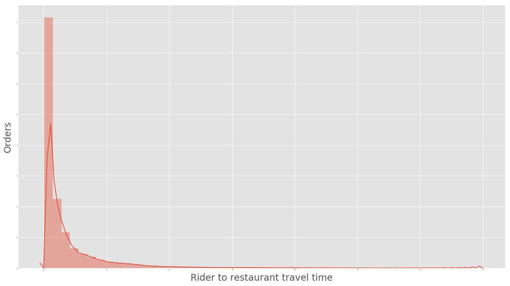
This data will violate the normality assumption of the t-test - although there are asymptotic justifications that the t-test is still valid even when our data is non-normal. Even if the t-test is valid, it will not be optimally powerful, there will exist alternative tests of the null hypothesis which have greater power to detect alternative hypotheses.
We can use the code presented before to perform a Monte Carlo power analysis. Here we are drawing our Monte Carlo samples from the empirical distribution of our previous data. Below, we show three power curves: one using Monte Carlo simulation with the t-test, one use the analytical power method for a t-test and one using Monte Carlo simulation with a Mann–Whitney U test. Prior to starting our experiment we can say that based on the empirical distribution of our data, our simulation says we need a sample size of 139k to use a t-test versus the 110k sample size the analytical method tells us. Here the analytical method underestimates the required sample size. A Mann-Whitney U test will require a smaller sample size (88k) but changes the hypothesis to testing if there is a difference in the distribution between variant and control. If we decide this hypothesis is the outcome we wish to test, we can use a smaller sample size.
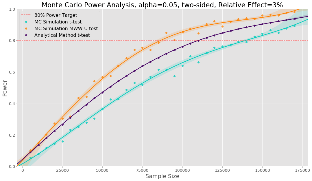
One of the strongest reasons we use Monte Carlo power analysis is that we can use the empirical distribution of our previous data to determine the right sample size and experimental analysis before running an experiment.
Power Analysis for Proportions
For proportion data, the method needs a slight adaptation. Below is an example for proportion data using multiple relative effects:
import numpy as np

from scipy.stats import binom
from statsmodels.stats.proportion import proportions_ztest

# Sample data would be actual data measured over a fixed period of time prior to our
# experiment. For illustration purposes here we have generated data from a normal
# distribution
sample_data = binom.rvs(1, 0.31518, size=900000)

base_conversion_rate = np.mean(sample_data)
sample_sizes = list(range(2000, 200000 + 1, 2000)) # Sample sizes we will test over
alpha = 0.05 # Our fixed alpha
sims = 250 # The number of simulations we will run per iteration
relative_effects = [1.01, 1.03, 1.05] # The list of relative effects we will test for
alternative = "two-sided" # Is the alternative one-sider or two-sided

power_dist = np.empty((len(sample_sizes), len(relative_effects), 2))
for i in range(0, len(sample_sizes)):
    for j in range(0, len(relative_effects)):
        relative_effect = relative_effects[j]
        N = sample_sizes[i]

        significance_results = []
        for k in range(0, sims):

            # # Randomly generate binomial data for variant and control with different
            # success probabilities
            sample_per_variant = int(np.floor(N/2))
            control_sample = binom.rvs(1, base_conversion_rate, size=sample_per_variant)
            variant_sample = binom.rvs(1, base_conversion_rate * relative_effect,
            	size=sample_per_variant)

            test_result = proportions_ztest(
            	count=[sum(variant_sample), sum(control_sample)],
            	nobs=[sample_per_variant, sample_per_variant], alternative=alternative)
            significance_results.append(test_result[1] <= alpha) # Test for significance
        # The power is the number of times we have a significant result
        power_dist[i,j,] = [N, np.mean(significance_results)]
        # as we are assuming the alternative hypothesis is true
The main difference is that we have to sample data from binomial distributions with two different success probabilities. The visualisation below shows the results for the three different relative effects tested:
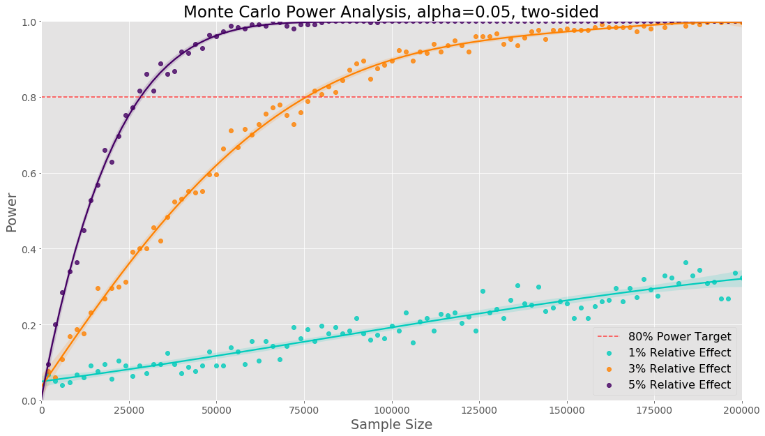
The sample sizes will be the same as we would obtain from an analytical method. If we only need a sample size for a single proportion, it will be less computation to use an analytical method. However in the next section we discuss multiple comparison, if we need a sample size in the case of a proportion metric with multiple comparisons the previous code example will be useful.
Power Analysis for Multiple Comparisons
In our final example, we will show how to use Monte Carlo simulation when we are running statistical tests on multiple metrics. Multiple comparisons occurs when we are running experiments with any of the following properties:
- Multiple metrics
- Multiple variants
- Segmenting by dimensions e.g. country, device
- Combinations of the above
The procedure shown below is almost identical in all these cases. The general method is within our simulation loop: run our statistical tests, correct for multiple comparisons, store if any of the tests were statistically significant after the correction, use these to calculate our power.
What do we mean by the power of an experiment when we have multiple comparisons? In the case with multiple metrics, our power could be any of the following two things:
- The probability that at least one metric is significant
- The probability that all the metrics are significant
If instead we had multiple variants (2 variants, 1 control), our power could be any of the following three things:
- The probability that at least one variant is significant
- The probability that all variants are significant
- The probability that the variants will be in the hypothesised ranking and all effects are significant. For example we hypothesise that variant 2 > variant 1 > control.
In the example below, we show how to use Monte Carlo simulation in the case of multiple metrics, creating the two power curves.
import numpy as np

from scipy.stats import norm, binom
from statsmodels.stats.weightstats import ttest_ind
from statsmodels.stats.multitest import multipletests

# Sample data would be actual data measured over a fixed period of time prior to our
# experiment. For illustration purposes here we have generated data from a normal
# distribution.
sample_mean_1 = 21.50
sample_sd_1 = 12.91
sample_data_1 = norm.rvs(loc=sample_mean_1, scale=sample_sd_1, size=80000)
sample_mean_2 = 6.51
sample_sd_2 = 3.88
sample_data_2 = norm.rvs(loc=sample_mean_2, scale=sample_sd_2, size=80000)

sample_sizes = range(2000, 80000 + 1, 1000) # Sample sizes we will test over
alpha = 0.05 # Our fixed alpha
sims = 1000 # The number of simulations we will run per sample size
relative_effect_1 = 1.035
relative_effect_2 = 0.98
alternative = "two-sided" # Is the alternative one-sided or two-sided

power_dist = np.empty((len(sample_sizes), 2, 2))
for i in range(0, len(sample_sizes)):
    N = sample_sizes[i]

    control_data_1 = sample_data_1[0:N]
    control_data_2 = sample_data_2[0:N]
    # Multiply the control data by the relative effect, this will shift the distribution
    # of the variant left or right depending on the direction of the relative effect
    variant_data_1 = control_data_1 * relative_effect_1
    variant_data_2 = control_data_2 * relative_effect_2

    significance_results_1, significance_results_2, significance_both,
    	significance_either  = [], [], [], []
    for j in range(0, sims):
        # Randomly allocate the sample data to the control and variant. Each sample is
        # ordered the same
        rv = binom.rvs(1, 0.5, size=N)
        control_sample_1 = control_data_1[rv == True]
        variant_sample_1 = variant_data_1[rv == False]
        control_sample_2 = control_data_2[rv == True]
        variant_sample_2 = variant_data_2[rv == False]

        # Use Welch's t-test, while our sample data has been generated using the
        # same variance, let's not assume this is true in general
        test_result_1 = ttest_ind(control_sample_1, variant_sample_1,
                                alternative=alternative, usevar='unequal')
        test_result_2 = ttest_ind(control_sample_2, variant_sample_2,
                                alternative=alternative, usevar='unequal')
        multi_comparision_result = multipletests([test_result_1[1], test_result_2[1]],
        	alpha=alpha,  method='h') # Use Holm correction
        metric_1_sig = multi_comparision_result[1][0] <= alpha
        metric_2_sig = multi_comparision_result[1][1] <= alpha
        significance_both.append(metric_1_sig and metric_2_sig)
        significance_either.append(metric_1_sig or metric_2_sig)
    power_dist[i,0,] = [N, np.mean(significance_both)]
    power_dist[i,1,] = [N, np.mean(significance_either)]
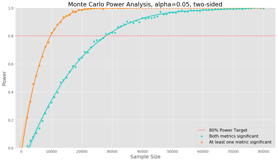
We show the two power curves in the plot below. In this case we need a much larger sample size to reach 80% power of both metrics being significant. If there was perfect positive dependence between the two metrics, the sample size needed would be the same. Using empirical data any dependence between the metrics will be taking into account. The relative effect for metric 1 was 3.5% and the relative effect for metric 2 was -2%.
The same code can be used in the case of multiple variants, segmenting by other dimensions, etc. We will need to change the logic inside of the simulation loop to compute the power curve of interest.
Introducing Echidna
As we can see from our examples, changing the assumptions of the experiment can lead to a lot of duplicated code. At Deliveroo we have packaged our experimental design and power analysis into an internal library called Echidna. This helps avoid code repetition and reduce analysis mistakes. We provide support for different types of experimental designs, different metric distributions and test statistics, multiple comparisons, etc. An example function call in Echidna for a block design experiment to obtain sample size is provided below:
def block_design_sample_size(self,
	metric_name: str,
	rel_effect_size: float=None,
	sample_sizes: np.array=None,
	alternative_hyp: str='two-sided',
	time_set_column: str='time_set') -> np.array:
	"""
	Experimental units are counterbalanced: half of units receive ABAB,
	half receive BABA, where B is treatment and A is control.
	"""
Our main reasons for developing Echidna were:
- We can hide implementation details and optimisations from end users, but anyone interested can still access the code. The Monte Carlo simulations are embarrassingly parallel but users should not need to reimplement this each time they run power analysis.
- We can encapsulate repetitive code into functions saving time and making analysis more readable.
- We avoid copy-paste coding which can lead to errors in analysis if people forget to update variables. This reduces the risk that we launch experiments but we have incorrectly calculated the required sample size.
- We have clear notebook examples of usage to make it easy for new joiners to pick it up.
Echidna is a collaborative effort across the Data Science team here at Deliveroo and is constantly being improved.
Summary
Monte Carlo simulation provides us with an extremely flexible way to run power analysis. The downsides are additional coding and time taken to run the simulation. Encapsulating our simulation methodology into a common library has allowed us to minimise any additional coding and create highly optimised implementations. Our default for very simple experimental designs is to still use analytical methods, but will switch to Monte Carlo simulation when required.
If you are interested in experimentation, power analysis or anything else in this blog post - take a look at our careers page for Data Science roles. We would love to hear from you!
About Daniel Nee

Dan is a Data Science Manager in the Algorithms team at Deliveroo building ranking and recommendations for our consumer facing products.
About Jamie Edgecombe

Senior Data Scientist and member of the Rider Online Experience team at Deliveroo.
About Jared Conway

Data scientist and member of the Growth team at Deliveroo for the past 2 years.